Diffusion-related meta data in Bruker files
Data sets
We have two data sets which have been acquired to the intent of determining the precise semantics of the diffusion-related parameters stored in Bruker files. They both comprise acquisitions with similar field of views, but with different slice geometry, both in the slice direction (axial, coronal, sagittal or oblique) and in the direction of the readout gradient within the slice plane (e.g. left-right or antero-posterior for an axial slice). The usual abbreviations for the human anatomical directions (LR, AP, HF) will be used in this document; even though the terms “head” and “feet” might be confusing for animals and readily replaced with respectively “rostral” and “caudal”, we will stick with the Bruker nomenclature and use “head” and “feet”.
The first data set is a phantom composed of three pieces of a strand of climbing rope (courtesy of Lucas Soustelle, ICube, University of Strasbourg-CNRS), each piece angled slightly differently. Three different acquisitions were performed, one sagittal, one coronal and one axial.
Series |
Orientation |
Readout |
Phase |
Slice |
|---|---|---|---|---|
5 |
Sagittal |
HF |
AP |
LR |
6 |
Coronal |
HF |
LR |
AP |
7 |
Axial |
LR |
AP |
HF |
The second data set is a rat head (courtesy of Chrystelle Po, ICube, University of Strasbourg-CNRS), with a total of seven acquisitions: two axial, two sagittal and two coronal, each set with two different readout directions, and an oblique slice prescription, close to axial.
Series |
Orientation |
Readout |
Phase |
Slice |
|---|---|---|---|---|
6 |
Axial (≈) |
LR |
AP |
HF |
8 |
Axial (≈) |
AP |
LR |
HF |
9 |
Sagittal |
HF |
AP |
LR |
10 |
Sagittal |
AP |
HF |
LR |
11 |
Coronal |
HF |
LR |
AP |
12 |
Coronal |
LR |
HF |
AP |
13 |
Oblique (close to axial) |
LR |
AP |
HF |
All meta-data are loaded from the method files in each series directory.
import glob
import os
import subprocess

import dicomifier
import nibabel
import numpy
import pandas
import tabulate

if not os.path.isdir("../../../tests/data/input"):
    subprocess.call(["../../../tests/download_data"])
root = "../../../tests/data"
bruker_paths = {
    "rope": os.path.join(root, "input", "20180818_175759_Rope_ChosenOne_1_2"),
    "rat": os.path.join(root, "input", "20171114_094354_Plateforme_R17_06_1_2")
}

series = {"rope": [5,6,7], "rat": [6,8,9,10,11,12,13]}

data = {}
for name in series:
    data[name] = {}
    for s in series[name]:
        data_set = dicomifier.bruker.Dataset()
        data_set.load(os.path.join(bruker_paths[name], str(s), "method"))
        data[name][s] = data_set
Units and coordinate systems
According to the official documentation of STB_InitDiffusionPreparation, PVM_DwDir and PVM_DwBvalEach are input parameters on which the user has control, while PVM_DwGradVec and PVM_DwEffBval are computed by Paravision.
The input parameters (PVM_DwDir and PVM_DwBvalEach) do not contain the actual diffusion scheme: the series number 5 of the rope data set has 13 volumes (including \(b=0\)), but PVM_DwDir only contains 12 values, and the full value of PVM_DwBvalEach is [1500] – obviously expressed in \(s/mm^2\).
On the other hand, the output parameters contain the actual diffusion scheme, including the \(b=0\) acquisition. However, the b-value is the effective one (i.e. taking into account the diffusion brought by the imaging gradients), which may confuse software expecting “exact” shells. Also note that the items in PVM_DwGradVec are not unit length: they are gradient amplitude, relative to the maximum gradient amplitude allowed by the system. Even though the norm of PVM_DwDir and PVM_DwGradVec differ, they are colinear.
The parameters of series number 5 of the rope data set is summarized below.
DwEffBval |
DwGradVec |
Norm |
DwDir |
Norm |
Colinear? |
|---|---|---|---|---|---|
36 |
[0.0, 0.0, 0.0] |
0 |
nan |
N/A |
|
1512 |
[0.05, 0.01, 0.2] |
0.21 |
[0.26, 0.07, 0.96] |
1 |
True |
1507 |
[-0.09, 0.03, 0.19] |
0.21 |
[-0.43, 0.14, 0.89] |
1 |
True |
1509 |
[-0.03, -0.12, 0.17] |
0.21 |
[-0.12, -0.56, 0.82] |
1 |
True |
1500 |
[0.15, -0.06, 0.13] |
0.21 |
[0.74, -0.27, 0.61] |
1 |
True |
1500 |
[0.08, 0.14, 0.13] |
0.21 |
[0.4, 0.66, 0.64] |
1 |
True |
1500 |
[-0.08, 0.16, 0.11] |
0.21 |
[-0.37, 0.75, 0.55] |
1 |
True |
1511 |
[-0.18, -0.02, 0.09] |
0.21 |
[-0.89, -0.09, 0.45] |
1 |
True |
1500 |
[-0.13, -0.15, 0.07] |
0.21 |
[-0.61, -0.72, 0.32] |
1 |
True |
1500 |
[0.08, -0.18, 0.08] |
0.21 |
[0.37, -0.85, 0.37] |
1 |
True |
1500 |
[0.19, 0.07, 0.05] |
0.21 |
[0.91, 0.32, 0.26] |
1 |
True |
1519 |
[0.03, 0.21, 0.02] |
0.21 |
[0.13, 0.99, 0.08] |
1 |
True |
1511 |
[-0.18, 0.1, 0.02] |
0.21 |
[-0.86, 0.5, 0.08] |
1 |
True |
Both for the rope and for the rat data set, the diffusion scheme is the same for all slice orientations. This, and the fact that PVM_DwGradVec are gradient amplitudes used directly in the pulse program, indicates that the diffusion gradient directions are expressed in slice coordinates (i.e. \((1,0,0)\) is the readout axis, and \((0,0,1)\) is the slice-selection axis, or slice normal).
Conversion to subject coordinates
In order to convert this data to subject coordinates (among others, used in DICOM and MRtrix), we need the coordinates of the imaging gradients in subject coordinates. The documentation of STB_UpdateTraj states that the parameter PVM_SPackArrGradOrient contains those values:
gradOrient: Gradient orientation matrix transferring between RPS (slice) and XYZ (object) coordinate system (note: XYZ represents AP-LR-HF)
However, looking at the values of PVM_SPackArrGradOrient, it seems that the XYZ coordinate system is instead the usual LR-AP-HF system. On the rope data set, the series 5, 6, and 7 are respectively sagittal, coronal and axial, and their respective gradient orientation matrices are:
5: \(\left(\begin{array}{rrr}0 & 0 & 1 \\ 0 & 1 & 0 \\ 1 & 0 & 0\end{array}\right)\)
6: \(\left(\begin{array}{rrr}0 & 0 & 1 \\ 1 & 0 & 0 \\ 0 & 1 & 0\end{array}\right)\)
7: \(\left(\begin{array}{rrr}1.0 & -0.0 & -0.0 \\ 0.0 & 1.0 & -0.0 \\ 0.0 & 0.0 & 1.0\end{array}\right)\)
It also seems that the matrix is either the transpose of the aforementioned transform for column-vectors, or is designed to be used with row-vectors.
With those two remarks, it is possible to define the directions of the diffusion gradient in subject coordinates by multiplying the transpose of PVM_SPackArrGradOrient by each normalized entry of PVM_DwGradVec.
directions_subject = {"rope": {}, "rat": {}}

for name, series in data.items():
    for s, d in series.items():
        grad_vec = get_array(d["PVM_DwGradVec"])
        # Avoid divide-by-zero
        grad_vec /= numpy.maximum(
            1e-20, numpy.linalg.norm(grad_vec, axis=1))[:,None]

        orientation = get_array(d["PVM_SPackArrGradOrient"])[0]
        # NOTE: use transpose, cf. previous remark
        directions_subject[name][s] = numpy.einsum(
            "ij,kj->ki", orientation.T, grad_vec)
Validation
We validate the transformation using a simple MRtrix-based pipeline:
Create a scheme file following MRtrix format
Estimate the diffusion tensors from the diffusion-weighted image and the scheme
Extract the first eigenvector from the tensor map
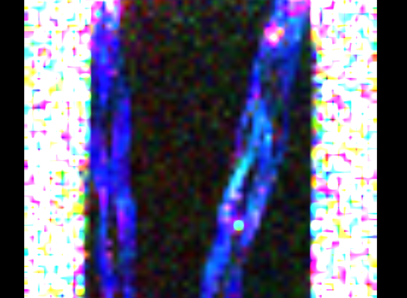
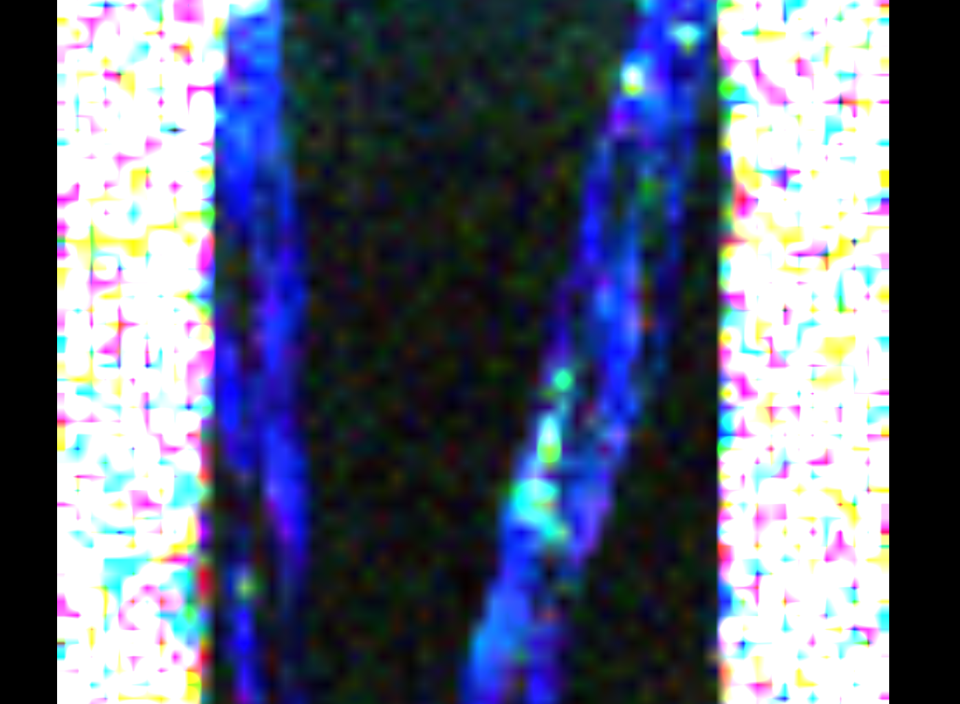
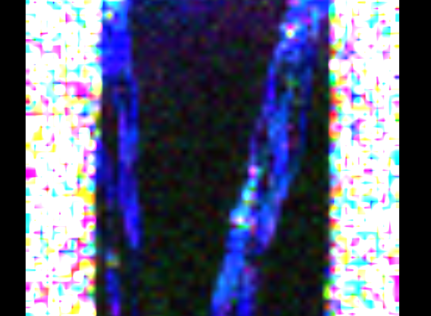
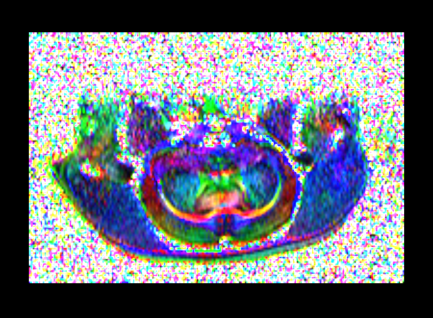
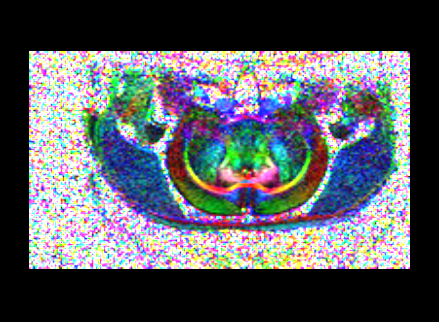
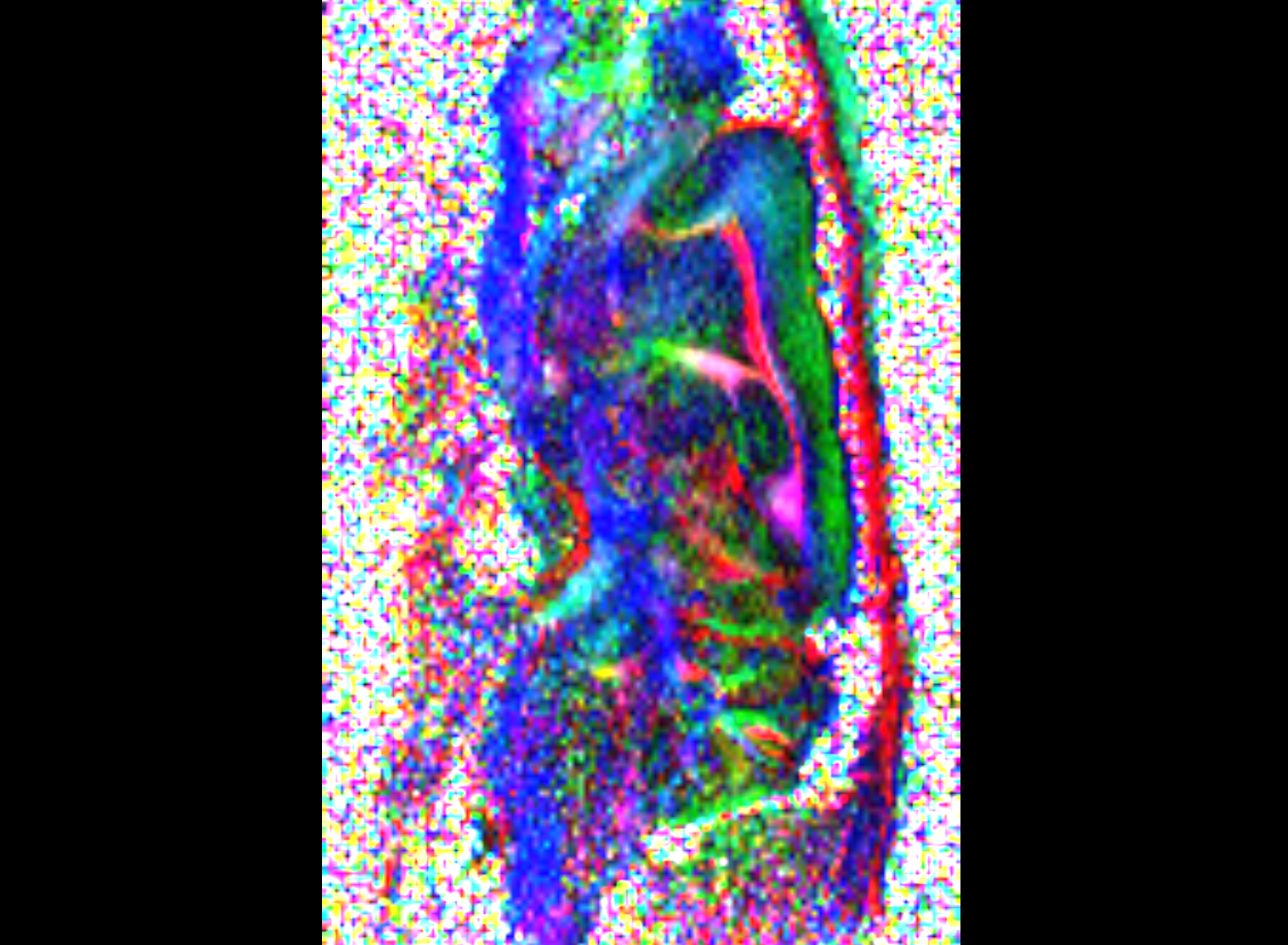
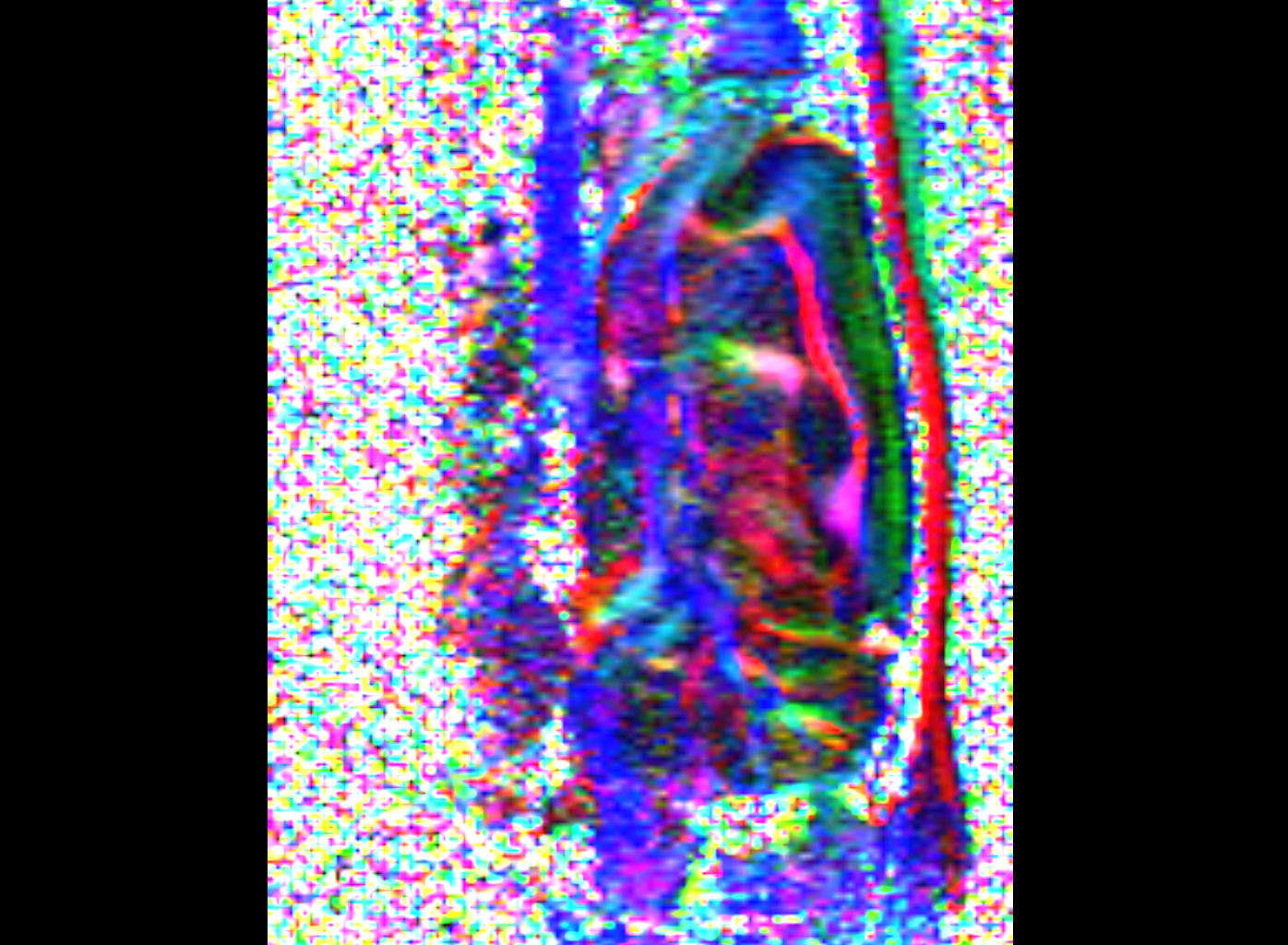
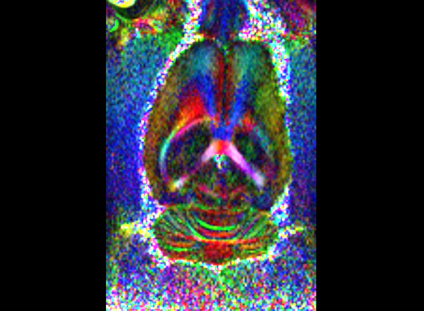
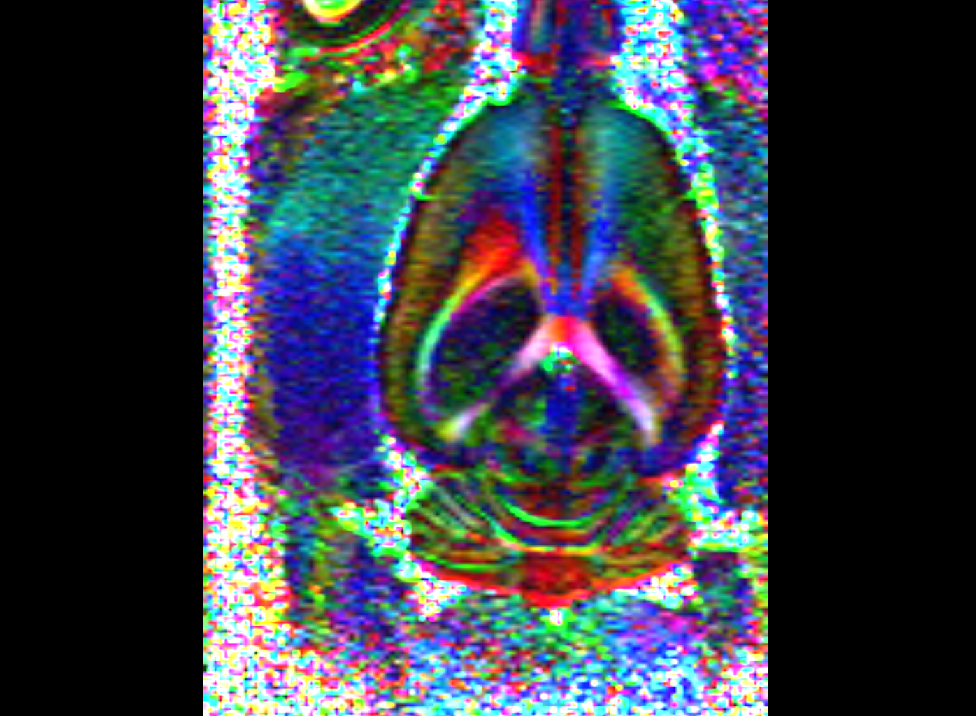
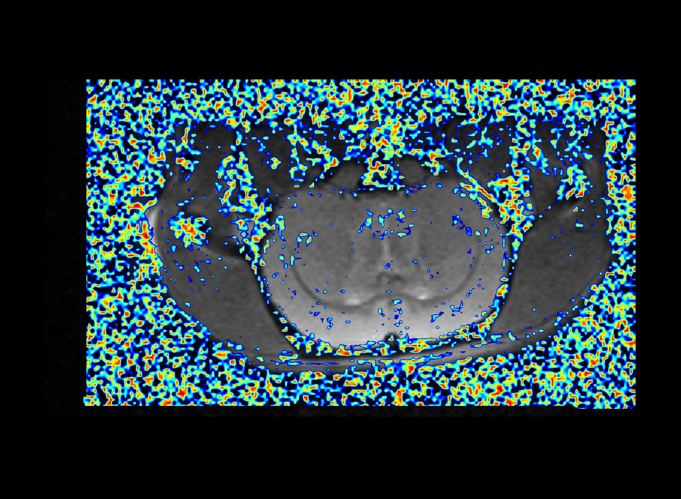
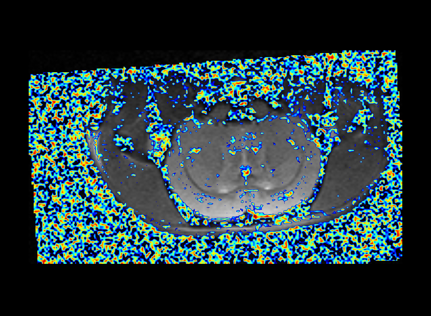
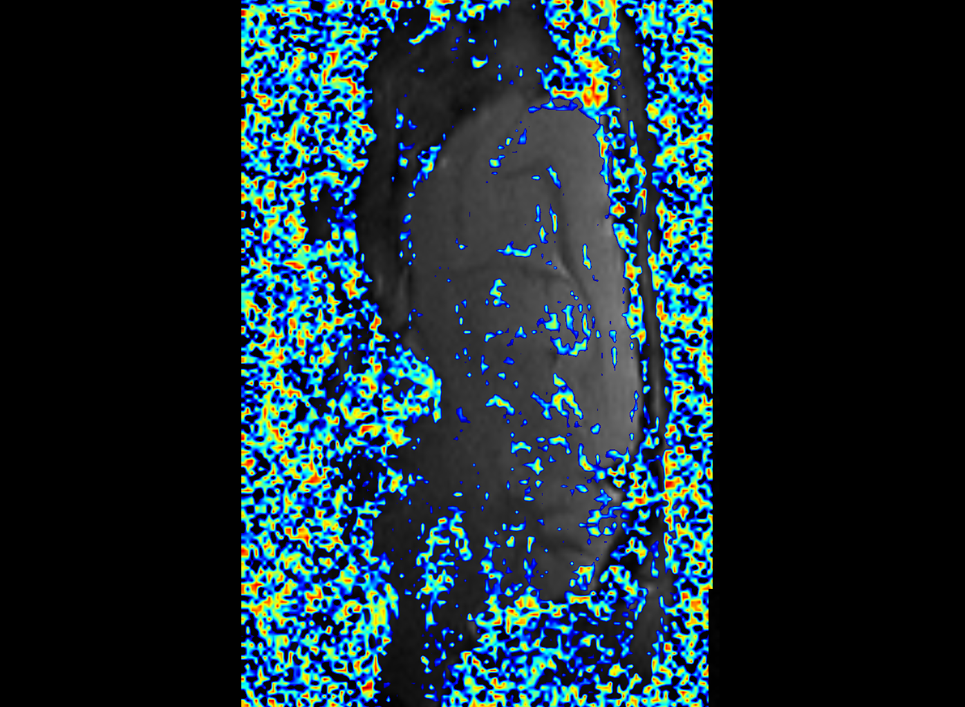
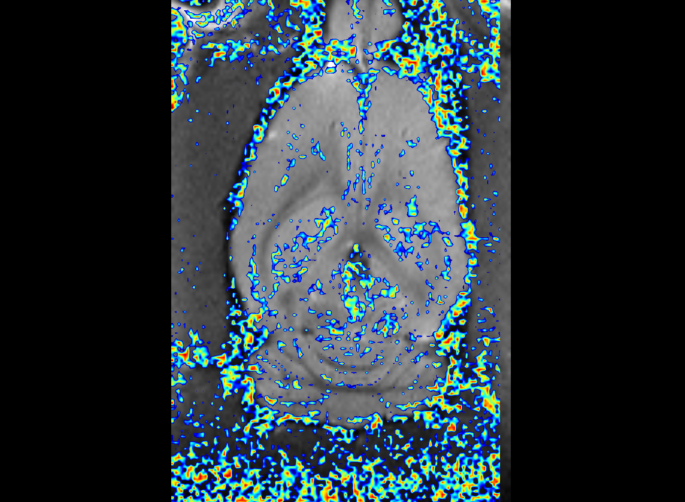
Qualitative
The following images show that the hue, indicating the principal direction of the direction tensor, is similar for the different series.
|
|
|
|
|
|
|
|
|
|
|
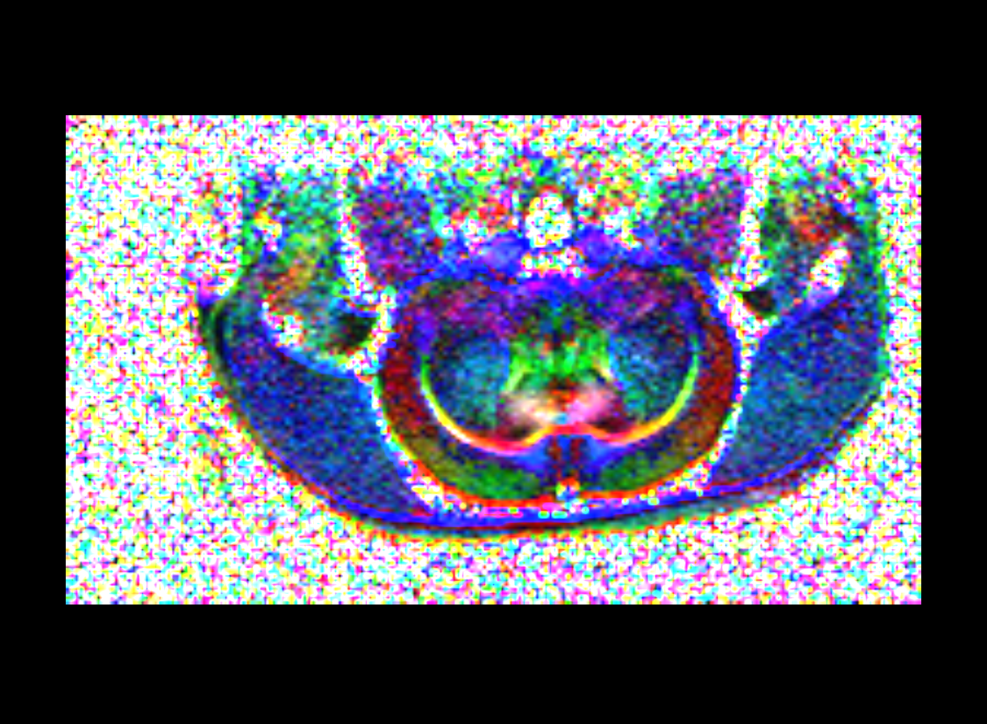
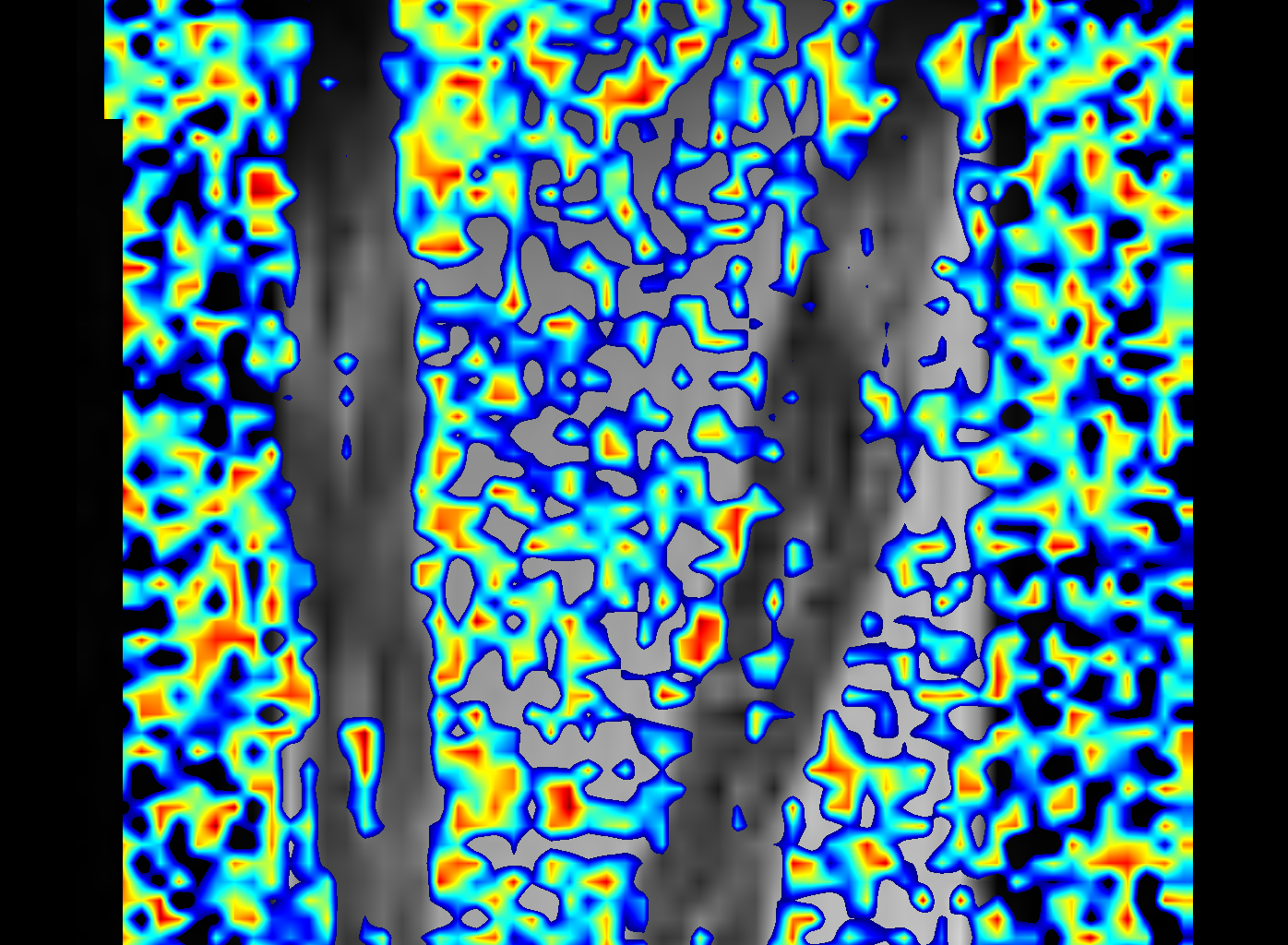
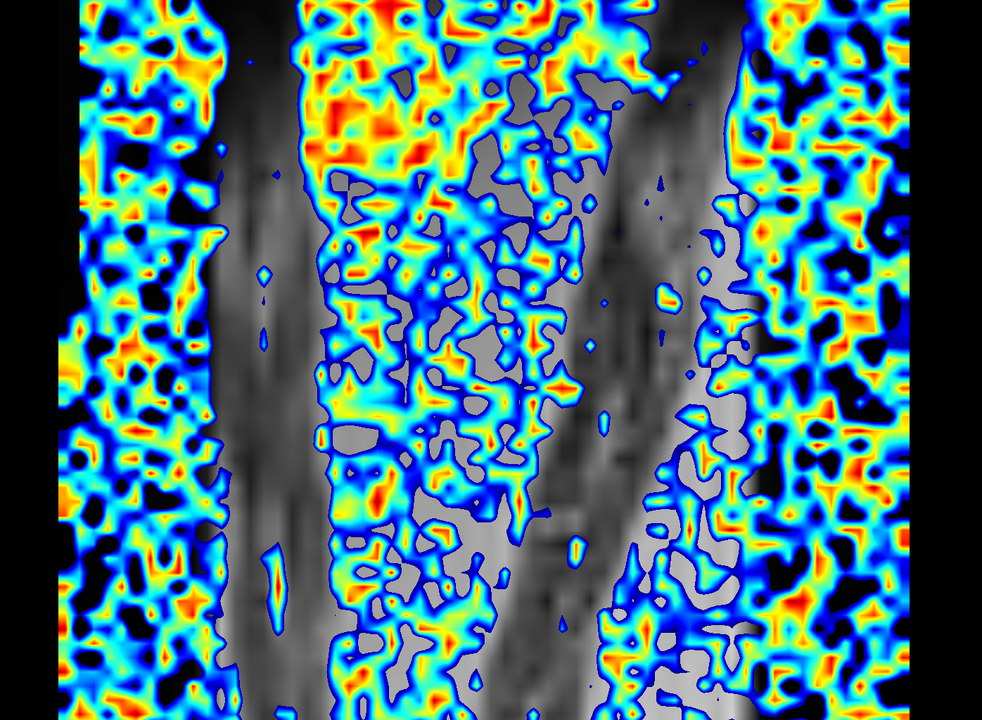
Quantitative
It is possible to go one step further and compute the angle between the principal eigenvector of a reference series (5 for the rope data set, 6, 9, and 11 for the rat data set) and the principal eigenvector of subsequent series (6 and 7 for the rope data set and respectively (8, 13), 10 and 12 for the rat data set). Due to some limitations in the data sets (one-dimensional object in the rope data set, high anisotropy of the voxels in the rat data set), we only focus on angles larger than 45 °; however, since the fields of view of the acquisitions are orthogonal to one another, any error would show as 90 ° angles between an image and its reference, and would appear at every voxel.
The following images show that, although there are large differences remaining, most of the object show similar principal directions, which validates the transform.
|
|
|
|
|
|